Professional Shunt Resistor Essentials for Accurate Current Measurement

Why do two current measurements on the same circuit sometimes differ by more than 10%? Often, the culprit is a poorly chosen shunt resistor. Getting accurate readings demands more than a low resistance value—it requires attention to thermal EMF, temperature stability, and construction. In this post, we break down the essentials of professional shunt resistors for precise current measurement, and show how Milliohm delivers solutions that meet these exacting standards.

Why a Shunt’s Tolerance Rating Is Only Half the Story

When engineers scan a shunt resistor datasheet, the first number they usually lock onto is the tolerance rating—±0.5%, ±0.1%, maybe even ±0.05% if budget allows. That figure, though, describes only the initial deviation from nominal at a single reference temperature, typically 25°C. It says nothing about what happens when the shunt heats up under load, when ambient temperature swings, or when the part ages over months and years. For a current-sensing resistor carrying tens of amps, the self-heating alone can push the resistance far beyond that neat catalog tolerance.

The real accuracy picture hinges on several secondary specifications. Temperature coefficient of resistance (TCR) tells you how much the resistance drifts per degree of temperature change—often a much larger error source than the initial tolerance. Thermal EMF from dissimilar metal junctions can add a small voltage offset that masquerades as current signal, especially in high-current, low-resistance shunts. Then there’s power coefficient, load life stability, and moisture absorption, all of which quietly erode precision over time. A shunt with 0.1% initial tolerance but a 100 ppm/°C TCR can easily show a 0.5% shift during normal operation, making that headline tolerance number only half the story—and sometimes less.

Thermal EMF: The Millivolt-Scale Error Hiding in Plain Sight

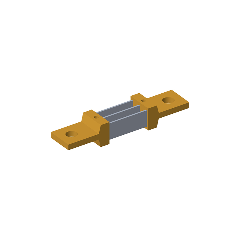
Every connection between two different conductors behaves like a tiny thermocouple. If the ends of that junction sit at different temperatures, a voltage appears—typically just a few microvolts per degree Celsius, but in precision systems it can combine with dozens of similar junctions to produce errors in the millivolt range. Thermal EMF rarely announces itself. It sits quietly in relay contacts, solder joints, and even the copper-to-gold interface on a PCB pad, waiting for a temperature gradient to turn a stable reading into a slow drift.

The trouble is that most circuit designs treat every node as if it were at a uniform temperature. In reality, power dissipated by nearby regulators, airflow from a fan, or even the warmth of an operator's hand can create gradients of a few degrees across a connector. At 10 µV/°C per junction, a 5°C difference across ten junctions adds up to 0.5 mV—enough to swamp a 16-bit ADC's least significant bits or shift a thermocouple measurement by several degrees. The error changes with time and environment, so it looks like random noise or a mysterious offset that calibration cannot fully remove.

Fighting thermal EMF starts with reducing both the number of junctions and the temperature differences across them. Use connectors and relays with low-thermal-EMF contacts, keep sensitive input pairs close together, and avoid placing them near heat sources. When a junction is unavoidable, matching materials on both sides and using thick copper planes to spread heat can cut the gradient dramatically. Some engineers even add short-term thermal shielding or slow the measurement rate to let the system settle. The goal is not to eliminate the physics—it is to make every junction see the same temperature, so the tiny thermocouples cancel instead of adding.

Four-Wire Kelvin Connections Eliminate Lead Resistance Artifacts

A two-wire measurement quietly folds the resistance of the test leads into the reading. For a 10 Ω resistor, that might be a minor irritation; for a 0.1 Ω shunt or a precision current-sense resistor, it becomes the dominant error. The meter cannot tell whether the voltage drop it sees comes from the device under test or from the copper between the terminals.

The four-wire Kelvin method splits the current path from the voltage sense path. One pair of leads carries the test current, while a second pair connects directly across the unknown resistance and feeds a high-impedance voltmeter. Because almost no current flows in the sense leads, their resistance contributes essentially no voltage drop. What the voltmeter reports is the true voltage across the device itself, not the device plus its wiring.

That separation makes lead length, contact quality, and even temperature-driven changes in lead resistance largely irrelevant. It is why low-resistance measurements, RTD probes, and shunt calibration setups routinely rely on Kelvin connections rather than accepting the artifacts a simpler hookup would introduce.

Manganin vs. Constantan: Matching Alloy to Measurement Range

Manganin and Constantan occupy overlapping niches in precision resistance work, but their practical measurement ranges diverge once temperature swings beyond a narrow band. Manganin, a copper-manganese-nickel alloy, delivers an exceptionally low temperature coefficient of resistance—often just a few parts per million per degree Celsius near room temperature. This makes it superb for metrology-grade resistors, shunts, and bridge circuits that operate in tightly controlled thermal environments. Push the temperature outside roughly 15 °C to 35 °C, however, and its TCR rises noticeably, so a Manganin-based sensor can drift if the ambient conditions are not stable. Constantan, by contrast, exhibits a higher but remarkably linear TCR across a broader span. If your measurement setup must tolerate industrial temperature fluctuations, Constantan often proves more predictable over the full operating range, even though its absolute stability at a single temperature is lower than Manganin's.

The choice looks different again when the range in question is mechanical strain or pressure rather than temperature. Constantan has long been the default foil strain gauge material for general-purpose testing, thanks to a favorable combination of gauge factor, fatigue life, and the ability to tailor its thermal output to match common structural materials like steel or aluminum. It handles static and slowly varying loads with repeatable accuracy across a wide strain range. Manganin, meanwhile, is prized in dynamic high-pressure experiments, such as shock wave and ballistic studies, where its resistance changes almost linearly with hydrostatic pressure up to several hundred kilobars. For that specialized measurement range—extreme, fast, and high-pressure—Manganin gauges remain indispensable, despite their limited utility in everyday strain work.

Matching the alloy to the measurement range thus requires weighing stability, linearity, and the environmental envelope together. If you need sub-microohm drift in a laboratory bridge or a precision current shunt, Manganin is the natural pick—provided you can keep the local temperature stable. If the transducer will spend its life on a bridge girder, inside an engine test cell, or on a load cell exposed to seasonal temperature swings, Constantan's rugged, wide-range behavior usually wins. Neither alloy is universally superior; the right answer depends on whether you are optimizing for a narrow band of ultra-high stability or a broad, less forgiving operating envelope where predictable moderate drift is acceptable.

Power Dissipation Limits and the Self-Heating Feedback Loop

The specified power dissipation limit of a semiconductor device often reads like a single number on a datasheet, but in practice it is a moving target shaped by local die temperature. As current flows through the channel or drift region, the dissipated energy raises the junction temperature, and that temperature change feeds back into the very parameters that determine power loss. A rise in temperature can lower threshold voltage, increase leakage current, or alter carrier mobility, each of which may push the device closer to thermal runaway. This self-heating feedback loop means the margin between a safe operating point and a destructive one can vanish faster than a simple derating curve suggests.

In silicon power MOSFETs, the positive temperature coefficient of RDS(on) is often treated as a stabilizing feature because it encourages current sharing among parallel die. Yet the same coefficient also means that conduction loss grows with temperature, so a hot-spot region can become a higher-loss region, reinforcing the thermal gradient unless the heat spreading is fast enough. Bipolar transistors and IGBTs show an even sharper feedback path: VBE falls with temperature while current gain can rise, so localized heating can draw more current into a single cell. In GaN HEMTs, dynamic on-resistance and current collapse under self-heating can create additional loss that does not appear in DC characterization, making the loop harder to predict.

Breaking or managing this feedback loop usually requires more than just choosing a larger package or a bigger heatsink. Designers need electro-thermal models that couple the device's temperature-dependent electrical behavior with transient thermal impedance, because the loop gain is frequency-dependent. A pulsed test sequence can reveal whether a given bias point drifts into an unstable region before the average case temperature exceeds the rated maximum. In practice, conservative derating based on worst-case junction temperature is a start, but the more reliable approach is to suppress the loop gain itself, through careful layout, thermal spreading, and operating point selection that keeps the device away from regions where positive feedback dominates.

Mechanical Strain and Solder Joint Effects on Long-Term Drift

Long-term drift in precision electronics rarely has a single root cause, but mechanical strain and solder joint behavior are often overlooked because they change slowly and leave no obvious trace in the moment. When a package is soldered to a board, the mismatch in coefficient of thermal expansion between silicon, copper, leadframe, and FR-4 creates residual stress. Over months or years, solder joints creep and stress-relax, redistributing that load into the die and surrounding materials. This gradual redistribution shifts the local stress state of sensitive analog or reference circuits, which can manifest as a few microvolts of offset drift or a slight change in gain that would be impossible to correlate with a visible solder crack under ordinary inspection.

Solder joints don't fail only by cracking; they also undergo microstructural coarsening and intermetallic growth at the interface. These changes alter joint stiffness and thermal conductivity, which changes how strain is transmitted into the package during each power or ambient temperature cycle. For a voltage reference or a precision amplifier, that means the die sees a slowly evolving mechanical boundary condition rather than a fixed one. In some cases, the drift direction reverses as the joint work-hardens locally and then partially recrystallizes, which produces the kind of non-monotonic drift curves that confuse accelerated life tests. The effect becomes more pronounced in lead-free solders, where tin-silver-copper alloys are stiffer and more prone to stress relaxation than traditional tin-lead joints.

A practical way to separate solder-related drift from purely electrical aging is to compare units with different mounting conditions—for example, a die attached with a high-temperature epoxy versus a fully reflowed BGA. If the drift signature changes with board thickness, solder volume, or underfill, the role of mechanical coupling becomes clear. Yet many datasheets only specify drift after a clean bake, which removes moisture but not the accumulated plastic strain in the joints. Field returns often show shifts that cannot be reproduced on freshly soldered samples until thermal cycling is applied, pointing back to the same conclusion: long-term stability is as much a mechanical system property as it is an electrical one.

FAQ

Conclusion

A shunt resistor’s tolerance rating often dominates early design conversations, but it only captures a narrow slice of real-world error. Thermal EMF generated at the junction between the resistance element and its copper terminations can introduce millivolt-scale offsets that quietly distort low-range measurements. Choosing the right alloy adds another layer: manganin delivers a very low temperature coefficient and excellent long-term stability for precision low-resistance shunts, while constantan becomes more practical in higher-resistance applications where its thermal behavior and cost profile fit the range. Even with a good alloy, the measurement path must include a four-wire Kelvin connection, otherwise lead and contact resistance artifacts will appear as false shunt voltage drops.

Power dissipation deserves just as much attention as electrical specifications. A shunt operating near its rated wattage enters a self-heating feedback loop—rising temperature changes the resistance, which alters the voltage drop, which further shifts the operating point. Derating the shunt and providing adequate thermal relief break that cycle before it erodes accuracy. Long-term stability is also shaped by mechanical factors: board flex, mismatched thermal expansion, and solder joint fatigue can induce microstrain that permanently shifts resistance. Rigid mounting, balanced pad geometry, and careful solder profiling help keep the shunt’s calibration intact over years of service. Precision current measurement is therefore a system-level discipline, not a single component choice.